Example 1. Replicate AUC Analysis of Hanley and McNeil (1982)
WMWprob is identical to the area under the curve (AUC) when using a receiver operator characteristic (ROC) analysis to summarize sensitivity vs. specificity in diagnostic testing in medicine or signal detection theory in
human perception research and other fields. Here we re-analyze the example used by Hanley and McNeil (1982) and again by Newcombe (2006).
 Screen-shot from Hanley and McNeil (1982).
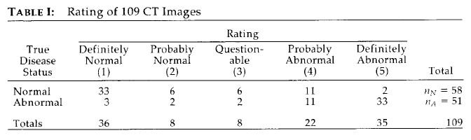
Storyline. Hanley and McNeil (1982) presented "illustrative data showing how a single reader (a radiologist) rated the computed tomographic (CT) images obtained in a sample of 109 patients with neurological problems."
Research question. How well do the radiologist's ratings of the images predict the true disease status of these patients? Let (Y.abnormal, Y.normal) be a pair of randomly selected scores from the two groups. There are 58*53 = 3074 unique pairings. Then
AUC = WMWprob = Prob[Y.abnormal > Y.normal] + Prob[Y.abnormal = Y.normal]/2.
To conclude that the image ratings are clinically useful, AUC should exceed 0.50 (just chance) by a substantial margin, say, AUC > 0.80. This is best addressed by computing the estimate and confidence interval.
Strictly speaking, this estimate and CI apply only to this single radiologist who read all images.
Creating the data.
> # .......... code block 1.1 ..........
> # Create the data.
> normal <- rep(1:5, c(33, 6, 6, 11, 2))
> abnormal <- rep(1:5, c( 3, 2, 2, 11, 33))
> Rating = c(normal,abnormal)
> TrueDiseaseStatus <- c(rep("Normal",length(normal)),
+ rep("Abnormal",length(abnormal)))
> # .......... end code block 1.1 ..........
Example 1a. Two-sided CI, [LCL, UCL]; p-value for tailored hypothesis.
The estimate and lower and upper confidence limits, [LCL, UCL], summarize the diagnostic accuracy of the CT readings as measured by the AUC. The goal to infer that AUC > 0.80 leads to the "essential" null hypothesis of H0: WMWprob = 0.80. (Testing H0: WMWprob = 0.50 is meaningless for this problem.)
> Ex1a <- WMW(Y=Rating, Group=TrueDiseaseStatus,
+ GroupLevel=c("Abnormal", "Normal"), H0.WMWprob=0.80)
*******************************************************
WMW: Wilcoxon-Mann-Whitney Analysis
Comparing Two Groups with Respect to an Ordinal Outcome
*******************************************************
Counts
**********************************************************************
Rating
TrueDiseaseStatus 1 2 3 4 5 Total
Abnormal 3 2 2 11 33 51
Normal 33 6 6 11 2 58
**********************************************************************
Sample Probability Distributions
**********************************************************************
Rating
TrueDiseaseStatus 1 2 3 4 5 Total
Abnormal 0.059 0.039 0.039 0.216 0.647 1.000
Normal 0.569 0.103 0.103 0.190 0.034 1.000
**********************************************************************
WMW Parameters
**********************************************************************
WMWprob = Pr[Rating{Abnormal} > Rating{Normal}] +
Pr[Rating{Abnormal} = Rating{Normal}]/2
WMWodds = WMWprob/(1-WMWprob)
**********************************************************************
Sample Sizes
***********************
Abnormal 51
Normal 58
***********************
************************************************************
Stochastic Superiority # of Pairs Probability
************************** ********** ***********
{Abnormal} < {Normal} 161 0.054
{Abnormal} = {Normal} 310 0.105
{Abnormal} > {Normal} 2487 0.841
Total: 2958 1.000
WMWprob = (2487 + 310/2)/2958 = 0.893
WMWodds = 0.893/(1 - 0.893) = 8.36
************************************************************
*****************************************************************
Estimate 0.95 CI* H0 p**
*****************************************************************
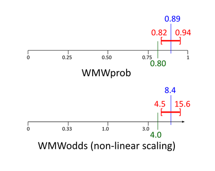
WMWprob 0.893 [0.817, 0.940] 0.800 0.020 (two-sided)
WMWodds 8.36 [4.47, 15.6] 4.00 0.020 (two-sided)
*****************************************************************
*Method based on Mee (JASA, 1990).
**P-value is always congruent with both confidence intervals.
Comments. These results agree with those for Data Set (a), Method 6 (Mee's method) in Table 1 of Newcombe (2006).
The estimated AUC (WMWprob) is 0.89; the 95% CI is [0.82, 0.94]. Because this CI excludes 0.80, the test of H0: WMWprob = 0.80 vs. H1: WMWprob ≠ 0.80 must have a congruent p-value less than 0.05; it is p = 0.020.
A distinct advantage of using only an estimate and a CI is that no null hypothesis needs to be set and no p-values become reported to the high proportion of people who fundamentally misunderstand them.
Using Newcombe's Method 3. The above results are based on Mee's method, the default. Using Method="Newcombe3" returns results that agree with Data Set (a), Method 3 in Table 1 of Newcombe (2006). Example 8 stress tests these two methods, providing strong evidence for favoring Mee's method.
Using the Hanley-McNeil standard error combined with Wilson's score method,
Using the Hanley-McNeil standard error combined with Wilson's score method,
> WMW(Y=Rating, Group=TrueDiseaseStatus, Method="Newcombe3",
+ GroupLevel=c("Abnormal", "Normal"), H0.WMWprob=0.80)
*****************************************************************
Estimate 0.95 CI* H0 p**
*****************************************************************
WMWprob 0.893 [0.810, 0.941] 0.800 0.031 (two-sided)
WMWodds 8.36 [4.27, 15.9] 4.00 0.031 (two-sided)
*****************************************************************
*Method 3 of Newcombe (Stat. in Med., 2006), which uses
the approximation of Hanley and McNeil (Radiology, 1990)
coupled with Wilson's (J. Am. Stat. Assn., 1927) scoring
CI method (instead of the Wald CI method).
**P-value is always congruent with both confidence intervals.
Example 1b. One-sided CI, [LCL, 1); p-value for tailored hypothesis.
It can be argued that the research question is primarily concerned with establishing a minimum for AUC. If so, using a CI of the form [LCL, 1] yields more cogent conclusions:
- The LCL in the [LCL, 1] interval will be nearer to the estimated AUC than in the [LCL, UCL] interval.
- Lower p-values give less support to H0: WMWprob ≤ 0.80 and thus greater support to H1: WMWprob > 0.80.
> Ex1b <- WMW(Y=Rating, Group=TrueDiseaseStatus,
+ GroupLevel=c("Abnormal", "Normal"), CI.type="L",
+ H0.WMWprob=0.80)
*****************************************************************
Estimate 0.95 CI* H0 p**
*****************************************************************
WMWprob 0.893 [0.831, 1.000] 0.800 0.010 (one-sided)
WMWodds 8.36 [4.93, Inf] 4.00 0.010 (one-sided)
*****************************************************************
*Method based on Mee (JASA, 1990).
**P-value is always congruent with both confidence intervals.
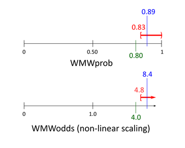
Comments. Compared to the two-sided LCL of 0.817 for AUC (Example 1a), the one-sided LCL of 0.831 is closer to the estimate of 0.893.
An honest and straightforward statement might be: The estimated AUC is 0.89 with a lower one-sided 95% confidence limit of 0.83. Note that "one-sided" is disclosed, but subtly, because the term too often elicits a dogmatic rebuke by those who follow the conventional wisdom that all CIs must be two-sided.
In the counterintuitive logic of p-value-ism, p = 0.010 reflects how much to disfavor H0: WMWprob ≤ 0.80 compared to H1: WMWprob > 0.80. However, the 95% LCL of 0.83 does that more directly and succinctly.
Bonus lesson. Note that, conveniently, p = 0.010 for H0: WMWprob ≤ 0.80 versus H1: WMWprob > 0.80. Accordingly, the 99% [LCL, 1] interval should be [0.800, 1.00]. And so it is:
> WMW(Y=Rating, Group=TrueDiseaseStatus, CI.level=0.99,
+ GroupLevel=c("Abnormal", "Normal"), CI.type="L",
+ H0.WMWprob=0.80)
Estimate 0.99 CI* H0 p**
*****************************************************************
WMWprob 0.893 [0.800, 1.000] 0.800 0.010 (one-sided)
