Toothpics()
Example 1: Basic ideas and comparisons
Example 2: Log-scaling works!
Example 4: How large can N be in a group?
Example 5: A 2 x 2 factorial design
Example 1: Basic ideas and comparisons
Example 2: Log-scaling works!
Example 4: How large can N be in a group?
Example 5: A 2 x 2 factorial design
Example 3: Other than log-scaling
What if your Y re-scaling is not log(Y)?
This example follows the edicts of Warton, D. I. and Hui, F. K. C. (2011). The arcsine is asinine: the analysis of proportions in ecology. Ecology, 92(1):3–10. (A great title, eh?)
A non-binomial proportion, Y (0 < Y < 1), is a measure that does NOT stem from observing S "successes" in N independent Bernoulli trials. Warton and Lui advocated using the logit transform, log(Y/(1-Y)). I am unaware of a set of terms for doing this, so let me propose these:
- yogit: log(Y/(1-Y)). Analogous to but quite different than the common logit, log(P/(1-P)); P = S/N, where S is a binomial(N, p) variate.
- yodds: Y/(1-Y) = exp(yogit). Analogous to odds = P/(1-P) = exp(logit).
- yodds ratio: ratio of two independent yodds. Analogous to the odd ratio.
- yoProp: yodds/(1 + yodds), the back transform a yodds value to give numbers in the friendly scaling of a proportion, 0 < yoProp < 1. Analogous to P = odds/(1 + odds).
To make their case, they analyzed raw data published by Moles and Westoby (2000) in which Y is the percentage loss of leaf area (LLA) on plants susceptible to herbivory (being eaten by animals of any kind, including insects). Those values show LLA ranging from virtually 0% to near 90% among different tree species.
Of course, people want to see the y-axis tick points and values expressed in terms of LLA not in terms of its yogit, e.g., LLA = 0.12 (12%) leaf loss is to be preferred over yogit(0.12) = log(0.12/0.88) = -1.99. But if the analysis will be done using yogit values, then the Y-axis should be scaled accordingly.
Science fiction
Background. Leaves of wiggly gum saplings are so favored by various insect larvae that median leaf loss area (LLA) is 50% (90% range: 20-90%). Thus, although most trees survive, their growth rate is too stunted to support profitable horticultural use.
Dr. Hugh Kaliptus has patented a new wiggly gum cultivar genetically motified to reduce herbivory by at least 20% so that, he claims, the median LLA is less than 30%. If so, this would promote faster growth. making the wiggly gum tree more commercially viable.
The Crainn Falsa Corporation (CFC) is considering purchasing Dr. Kaliptus's patent. But first they conducted their own study to test his claims.
Design and statistical method. In mid-March 2015 (before larvae were hatching), 32 healthy, two-year-old "natural" wiggly gum (group "N") saplings and 32 healthy same-age genetically modified saplings (group "GM") were transplanted to an open field prepared and maintained to be ideal as is practical for the wiggly gum. The 8 x 8 layout was:
N GM N GM N GM N GM
GM N GM N GM N GM N
N GM N GM N GM N GM
GM N GM N GM N GM N
N GM N GM N GM N GM
GM N GM N GM N GM N
N GM N GM N GM N GM
GM N GM N GM N GM N
In mid-July, each sapling was measured for LLA, yielding values with a minimum of 0.01 (even when it appeared to be 0.00) to a maximum of 0.87.
Primary analysis. CFC's statistician, Ms. Cliste Bean, has read Warton and Lui (2011) and wisely decided to use the estimates and 99% CI of the mean difference in logit(LLA) = log(LLA/(1-LLA)), as obtained using the Welch t statistic. For better communication, she will transform these to yodds ratios. This cannot be converted to a CI for the difference in mean LLA values.
Data generation. The Rfunc file for Toothpics() gives all code used to generate the data.
Toothpics() and related statements, Graphic 3
yogitLLA <- log(LLA/(1-LLA))
mean.yogitLLA <- tapply(yogitLLA, cultivar, mean, na.rm=T)
(yoProbLLA <- 1/(1 + exp(-mean.yogitLLA)))
GM N
0.1478899 0.5077580
meanvalues=format(yoProbLLA,digits=3)
qtemp <- tapply(LLA, cultivar, HDquantile, Tau=c(0.50, 0.80), Print=FALSE)
qvalues <- matrix(format(c(qtemp$GM$Q, qtemp$N$Q),digits=3),2,2,byrow=TRUE)
yticks.char=c("0.003", "0.01", "0.05", "0.10", "0.20", "0.40", "0.60", "0.80",
"0.90", "0.95", "0.99", "0.997")
yticksat <- log(as.numeric(yticks.char)/(1-as.numeric(yticks.char)))
PlotDirector(PlotSize=list(w=5.5, h=5), CloseOld=TRUE)
yogitLLA.jit <- FitterJitter(Y=yogitLLA, Groups=cultivar,Factor=3)$y.jit
Toothpics(
Title=paste("How Much Does the Generically",
"\nModified Cultivar Reduce Herbivory?"),
Y=yogitLLA.jit,
RawY=yogitLLA,
YLabel="Leaf Loss Area\n(LLA; yogit scaling)",
Group=cultivar,
GroupLevels=c("GM","N"), # Required!
YTickDigits=2,
YTicksAt=yticksat,
YTickLabels=yticks.char,
MeanValues=meanvalues,
QValues=qvalues,
YAxisLimits=log(c(0.006,0.994)/(1-c(0.006,0.994))),
GroupLabel="Wiggly Gum Cultivar",
GroupNames=c("Genetically\nModified", "Natural\n"),
Quantiles=c(0.50,0.80),
TPLength=1.4
)
Graphic 3
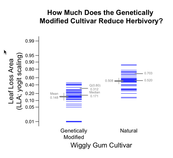
Toothpics() graphic 3.
Computational analysis
(ttest.3 <- t.test(yogitLLA ~ cultivar, conf.level=0.99))
Welch Two Sample t-test
data: yogitLLA by cultivar
t = -6.691, df = 59.69, p-value = 8.579e-09
alternative hypothesis: true difference in means is not equal to 0
99 percent confidence interval:
-2.491019 -1.073546
sample estimates:
mean in group GM mean in group N
-1.75124770 0.03103455
(yodds.est <- exp(ttest.3$estimate))
mean in group GM mean in group N
0.1735573 1.0315211
# yodds ratio: 0.1735573/1.0315211 = 0.1682538
(yoProb <- yodds.est/(1 + yodds.est))
mean in group GM mean in group N
0.1478899 0.5077580
# These values appear on graphic, too.
(yoddsratio.est <- exp(ttest.3$estimate[1]-ttest.3$estimate[2]))
0.1682537
(yoddsratio.ci <- exp(ttest.3$conf.int))
[1] 0.08282553 0.34179453
attr(,"conf.level")
[1] 0.99
Summary statement
Using the logit-transform approach, the estimated proportion of LLA (yoProb) was 15% for the genetically modified cultivar versus 51% for natural, giving yodds of 0.17 vs. 1.03 for a yodds ratio of 0.17. The 99% confidence interval was [0.08, 0.34]. The graphic and the computational statistics indicate convincingly that the GM cultivar is markedly less susceptible to herbivory.
