HDquantile()
Computes:
Example 4 is a small Monte Carlo study that begins to answer:
Current version: 03 January 2016.
Download HDquantile.Rfunc170103.R
Computes:
- Estimates of the quantiles (percentiles) of a distribution using the Harrell-Davis (HD) method. Also returns the Harrell-Davis weights used for those estimations.
- Confidence intervals for quantiles using the bias-corrected accelerated (BCa) percentile bootstrap method of Efron and Tibshirani.
Example 4 is a small Monte Carlo study that begins to answer:
- How does the HD method compare to R's default ordinary method for estimating quantiles?
- What is the actual coverage level versus the nominal coverage level for the BCa bootstrap confidence intervals?
Current version: 03 January 2016.
Download HDquantile.Rfunc170103.R
 Harrell, F. E. and Davis, C. E. (1982). A new distribution-free quantile estimator. Biometrika, 69(3):635–640.
Introduction
In his seminal 1908 Biometrika article on "The Probable Error of a Mean," William S. Gosset ("Student") wrote, "In a greater number of cases the [research] question finally turns on the value of a mean, either directly, or as the mean difference between the two quantities." A century later, t-tests, ANOVA, and their various extensions for estimating and making inferences on expected values still occupy a prominent place in our statistical toolboxes, including mine.
On the other hand, many research questions are better addressed by focusing on a specific quantile (percentile) of the distribution and analyzing how it differs between groups. I now prefer the Harrell-Davis quantile estimator (Harrell, F. E. and Davis, C. E. (1982). A new distribution-free quantile estimator. Biometrika, 69(3):635-640), and I hope to soon propose a general "analysis of quantiles" (ANOQU) method that teams it with the bias-corrected accelerated percentile (BCa) bootstrap algorithm of Efron and Tibshirani (1993) to compare quantiles (including, medians, of course) in a way isomorphic with ANOVA.
HDquantile() takes the first step: A tool to obtain better quantile estimates and a sound way to obtain associated confidence intervals.
Arguments
Y=NULL
Tau=0.50
CI.level=0.95
B=2000
N=NA
Seed=1234567,
Print=TRUE
Y=NULL
- Numeric variable, may have NAs. If Y=NULL, then giving N= and Tau= will return only HD weights; see Example 3.
Tau=0.50
- Quantile levels. For example, to estimate the median and 80th percentile, use Tau=c(0.50,0.90).
CI.level=0.95
- Level for bootstrap-based confidence interval. Use CI.level=NA to suppress.
B=2000
- Number of bootstrap samples. B=0 suppresses computing bootstrap estimates and bootstrap-based confidence intervals.
N=NA
- Sample size. Only used if Y=NULL. For example, to get the HD weights for N=10 and Tau=0.80, use HDquantile(Tau=0.80, N=10). Only one {N, Tau} combination allowed.
Seed=1234567,
- Seed for bootstrap resampling. This induces reproducibility, so that identical analyses of the same data produces the same results. But it also resets the seed for the whole environment. Thus when doing simulations, each trial may give identical results. To avoid this, use Seed=NA.
Print=TRUE
- =FALSE will suppress printing. Needed for Monte Carlo simulations; see Example 4.
Objects Returned
A list containing:
$Q Regular HD estimates of quantiles; vector of length(Tau)
$Q.boot Mean of B bootstrapped HD estimates; vector of length(Tau)
$CI Confidence limits for quantiles; matrix of length(Tau) rows by 2 columns
$HDwts Harrell-Davis weights; matrix with length(Tau) rows by N columns
Note: If Y=NULL, only $HDwts is returned. See Example 3.
Harrell-Davis quantile estimation
Let {y} = y[1] ≤ y[2] ≤ ... ≤ y[n] be a sample of n independent sorted observations (i,e. the n order statistics) from the same underlying continuous distribution of no specific form. We seek to use {y} to estimate the 100τ-th quantile (percentile), Q(τ): Prob[y ≤ Q(τ)] = τ, where τ (tau) is within (0, 1). For the median (τ = 0.50), when N is odd, the ordinary estimate is the middle value, y[n/2 + 1]. For N even, we take the average of the two middle values. For other quantiles (τ ≠ 0.50), the ordinary estimator is a weighted average of the two observations closest in rank corresponding to τ. For example, with N=10, the default ordinary estimator forQ(0.80) in R's core quantile() function is ord.quantile(0.80; N=10) = 0.80y[8] + 0.20y[9]. For Q(0.95), it is ord.quantile(0.95; N=10) = 0.45y[9] + 0.55y[10].
HD estimation uses a weighted average of all the observations with the weights set by a complex function dependent only on τ and n. There is no point to detailing this here, but it is worthwhile to compare two sets of HD weights for N=10.
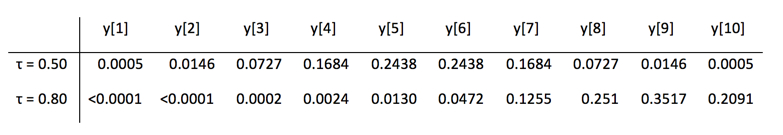
HD weights for N = 10 and τ = 0.50 (the median) and τ = 0.80.
Thus, the HD estimator for the median of 10 observations is 0.0005y[1] + ... + 0.2438y[5] + 0.2438y[6] + ... + 0.0005y[10].
Importantly, unless all N elements of Y are equal, HDquantile(Y, Tau) is a smooth, strictly increasing function of Tau, which is not true for the ordinary estimators (thus compromising their suitability for bootstrapping). When Y quantifies a continuous variable like pain level using an ordered categorical rating scale of 0, 1, 2, ... 10, the estimate of Q[τ+ε] will exceed that of Q[τ] for any arbitrarily small positive ε. Of course, strictly speaking, even our most "continuous" Y data are ordered categorical. We see blood pressure values of 146/94 mm Hg, not 145.986.../93.756...
BCa-bootstrap confidence intervals
After reviewing what experts in bootstrapping have recommended and doing some Monte Carlo investigations myself, I chose to construct confidence limits using the bias-corrected accelerated (BCa) percentile bootstrap method detailed in Efron, B. and Tibshirani, R. J. (1993). An Introduction to the Bootstrap. Chapman and Hall. Example 4 below summarizes a Monte Carlo study based on 5000 trials sampling N=51 from a logNormal distribution. The estimated coverage for a 95% CI for Q(0.50) was 0.938, with a 95% CI for the coverage rate of [0.937, 0.949]. This is excellent for a method that makes no assumptions about the parent distribution. Then again, it is only one situation. Other scenarios may be investigated by modifying Example 4.
Examples
Example 1
Starting simple, I generated 51 observations of Y ~ logNormal such that the true mean and standard deviation of log(Y) were 5 and 1.5. The true median and 0.80 of Y are 148.4 and 524.5. See Rfunc file for complete code.
HDquantile() statement
HDquantile(Y, Tau=c(0.50, 0.80), CI.level=0.90)
Result
Harrell-Davis Quantile Estimation
-----------------------------------
Variable (Y): Y
Quantile levels (Tau): 0.50 0.80
HD quantile estimates: 154 481
Bootstrap HD estimates: 155 495
Confidence intervals (level = 0.90)
lower upper
50% 89.9 246.2
80% 339.7 742.7
Example 2
This simulates data inspired by Figure 1 in Ramakrishna et. al. Amylase-resistant starch plus oral rehydration solution for cholera. New England Journal of Medicine, 2000; 342:308-13. See Rfunc file for code.
From the abstract (fictionalized slightly):
This study randomly assigned 48 adolescents and adults with cholera
to treatment with standard oral rehydration therapy only (15 patients),
standard therapy plus 50 g of rice flour per liter of oral rehydration
solution (16 patients), or standard therapy plus 50 g of high-amylose
maize starch, an amylase-resistant starch, per liter of oral rehydration
solution (17 patients). A primary end point was length of time to the first
formed stool.
HDquantile() statement and related code
HDq <- tapply(TimeFirstStool, Treatment, HDquantile,
Tau=c(0.50, 0.80), Print=FALSE)
TrtLevel <- c("StandardOnly","+RiceFlour","+ResistantStarch")
for (i in 1:3) {
cat("\n","***",TrtLevel[i],"***","\n")
print(round(HDq[[i]][["Q"]],1))
print(round(HDq[[i]][["CI"]],1))
}
Results
*** StandardOnly ***
50% 80%
55.4 73.0
lower upper
50% 47.4 66.1
80% 59.8 86.5
*** +RiceFlour ***
50% 80%
73.4 88.7
lower upper
50% 59.9 83.5
80% 79.1 95.2
*** +ResistantStarch ***
50% 80%
93.0 120.4
lower upper
50% 74.5 112.2
80% 106.3 138.3
Example 3
Obtaining HD weights for N = 10 and Tau = 0.50 and 0.80 (as discussed above).
HDquantile() statement
(HDw = round(HDquantile(N=10,Tau=c(0.50,0.80)),4))
Results
Tau 1 2 3 4 5 6 7 8 9 10
50% 5e-04 0.0146 0.0727 0.1684 0.2438 0.2438 0.1684 0.0727 0.0146 0.0005
80% 0e+00 0.0000 0.0002 0.0024 0.0130 0.0472 0.1255 0.2510 0.3517 0.2091
HDquantile() statement
(HDw = round(HDquantile(N=10,Tau=c(0.50,0.80)),4))
Results
Tau 1 2 3 4 5 6 7 8 9 10
50% 5e-04 0.0146 0.0727 0.1684 0.2438 0.2438 0.1684 0.0727 0.0146 0.0005
80% 0e+00 0.0000 0.0002 0.0024 0.0130 0.0472 0.1255 0.2510 0.3517 0.2091
Example 4
A "preliminary" Monte Carlo study.
This returns to the situation of Example 1, sampling N=51 observations from a LogNormal distribution that has a true median of 148.4. Here we generated 5000 such samples and analyzed each with each with the default settings for the median() function and with HDquantile (Y, Tau=0.50). Questions:
Code
See Rfunc file, about 40 statements.
Results
Prob.HDcloser: probability that HD median is closer than ordinary median to the true median
[CLim95Lo, CLim95Hi]: 95% confidence limits for Prob.HDcloser
Prob.HDcloser CLim95Lo CLim95Hi
0.552 0.538 0.566
==============================================================
MAD.HD: Mean absolute deviation of HD median from the true median
MAD.Ordinary: Mean absolute deviation of ordinary median from true median
gmeanHDvsOrd: Geometric mean of HD-vs-ordinary absolute error,
absolute deviation of HD median from true median
HDvsOrd= -----------------------------------------------------------
absolute deviation of ordinary median from true median
HDvsOrd < 1 favors HD.
Note. We need to use the geometric mean so that HDvsOrd = 4/5 (say) is the opposite of HDvsOrd = 5/4. (Even some experienced professional statisticians "forget" to do this.)
[CLim95Lo, CLim95Hi]: 95% confidence limits for gmeanHDvsOrd
MAD.HD MAD.Ordinary gmeanHDvsOrd CLim95Lo CLim95Hi
31.1 31.8 0.968 0.942 0.994
==============================================================
CIcoverage: Estimated coverage rate for 95% CI
[CLim95Lo CLim95Hi]: 95% confidence limits for CIcoverage.
CIcoverage CLim95Lo CLim95Hi
0.943 0.937 0.949
What does this limited study tell us? With this logNormal parent and N=51, about 55% of the HD estimates were closer to the true median than was the estimate given by median()-- here, the 26th largest observation.
Regarding absolute deviations from the true value, the HD method had less of this variability: gmeanHDvsOrd = 0.968 (< 1) with a "significant" 95% CI of [.942, 0.994].
In this situation, the HD method "wins."
For the serious/curious learner, see what happens when you change the N to be lower or higher than 51. Using Ntrials=1000 should be sufficient.
On my MacBook Pro 2.6 GHz Intel Core i7, running N=300 and Ntrials=1000 took 2.2 minutes. Is that long? Each trial involves B = 2000 bootstrap replications, so, in effect, there were 2,000,000 datasets created, sorted, and analyzed by both HD and ordinary method.
The results:
Prob.HDcloser CLim95Lo CLim95Hi
0.53 0.499 0.561
MAD.HD MAD.Ordinary gmeanHDvsOrd CLim95Lo CLim95Hi
12.5 12.7 1.01 0.965 1.06
CIcoverage CLim95Lo CLim95Hi
0.954 0.941 0.967
This is a solid performance by the HD quantile method with BCa bootstrap CIs.
On my Macbook, computing a single HD estimate and CI for N = 300 is virtually instantaneous.
This returns to the situation of Example 1, sampling N=51 observations from a LogNormal distribution that has a true median of 148.4. Here we generated 5000 such samples and analyzed each with each with the default settings for the median() function and with HDquantile (Y, Tau=0.50). Questions:
- How do the HD estimates of the median compare to the ordinary method for estimating the median? Which estimator tends to be closer to the true value?
- What is HDquantile's actual coverage level for its confidence interval (BCa percentile bootstrapping) versus the nominal coverage level?
Code
See Rfunc file, about 40 statements.
Results
Prob.HDcloser: probability that HD median is closer than ordinary median to the true median
[CLim95Lo, CLim95Hi]: 95% confidence limits for Prob.HDcloser
Prob.HDcloser CLim95Lo CLim95Hi
0.552 0.538 0.566
==============================================================
MAD.HD: Mean absolute deviation of HD median from the true median
MAD.Ordinary: Mean absolute deviation of ordinary median from true median
gmeanHDvsOrd: Geometric mean of HD-vs-ordinary absolute error,
absolute deviation of HD median from true median
HDvsOrd= -----------------------------------------------------------
absolute deviation of ordinary median from true median
HDvsOrd < 1 favors HD.
Note. We need to use the geometric mean so that HDvsOrd = 4/5 (say) is the opposite of HDvsOrd = 5/4. (Even some experienced professional statisticians "forget" to do this.)
[CLim95Lo, CLim95Hi]: 95% confidence limits for gmeanHDvsOrd
MAD.HD MAD.Ordinary gmeanHDvsOrd CLim95Lo CLim95Hi
31.1 31.8 0.968 0.942 0.994
==============================================================
CIcoverage: Estimated coverage rate for 95% CI
[CLim95Lo CLim95Hi]: 95% confidence limits for CIcoverage.
CIcoverage CLim95Lo CLim95Hi
0.943 0.937 0.949
What does this limited study tell us? With this logNormal parent and N=51, about 55% of the HD estimates were closer to the true median than was the estimate given by median()-- here, the 26th largest observation.
Regarding absolute deviations from the true value, the HD method had less of this variability: gmeanHDvsOrd = 0.968 (< 1) with a "significant" 95% CI of [.942, 0.994].
In this situation, the HD method "wins."
For the serious/curious learner, see what happens when you change the N to be lower or higher than 51. Using Ntrials=1000 should be sufficient.
On my MacBook Pro 2.6 GHz Intel Core i7, running N=300 and Ntrials=1000 took 2.2 minutes. Is that long? Each trial involves B = 2000 bootstrap replications, so, in effect, there were 2,000,000 datasets created, sorted, and analyzed by both HD and ordinary method.
The results:
Prob.HDcloser CLim95Lo CLim95Hi
0.53 0.499 0.561
MAD.HD MAD.Ordinary gmeanHDvsOrd CLim95Lo CLim95Hi
12.5 12.7 1.01 0.965 1.06
CIcoverage CLim95Lo CLim95Hi
0.954 0.941 0.967
This is a solid performance by the HD quantile method with BCa bootstrap CIs.
On my Macbook, computing a single HD estimate and CI for N = 300 is virtually instantaneous.
