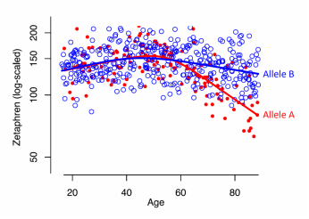
 iRCS fitting comparing f(X) between two groups. See Example 3.
iRCSplines()
Rfunc tested and released, but this webpage is far from done.
Makes predictor variables, X.1, X.2, ..., X.(K-1) to build a K-knot interpretable restricted cubic spline (iRCS) model, Y ~ f(X), where X and Y are, in theory, continuous.
f(X) = beta.0 + beta.1*X.1 + beta.2*X.2 + ... + beta.(K-1)*X.(K-1).
The X.i predictor variables are wholly not intuitive, but every beta coefficient provides direct and useful information about f(X). Other predictors can be added, including terms that compare f(X) among groups (interaction effects).
Example 1 teaches the anatomy of the basic 4-knot iRCS model. Changing the values of its parameters gives users hands-on experience in manipulating the function's shape. Example 2 demonstrates how to use iRCS model to compare the Y ~ f(X) relationships of two groups.
Rfunc tested and released, but this webpage is far from done.
Makes predictor variables, X.1, X.2, ..., X.(K-1) to build a K-knot interpretable restricted cubic spline (iRCS) model, Y ~ f(X), where X and Y are, in theory, continuous.
f(X) = beta.0 + beta.1*X.1 + beta.2*X.2 + ... + beta.(K-1)*X.(K-1).
The X.i predictor variables are wholly not intuitive, but every beta coefficient provides direct and useful information about f(X). Other predictors can be added, including terms that compare f(X) among groups (interaction effects).
- Current version released 12 May 2016. Windows and Linux not checked yet, but should not be a problem.
- Download iRCSplines.Rfunc160512.R
Example 1 teaches the anatomy of the basic 4-knot iRCS model. Changing the values of its parameters gives users hands-on experience in manipulating the function's shape. Example 2 demonstrates how to use iRCS model to compare the Y ~ f(X) relationships of two groups.
Arguments
X = <numeric object>
Nknots = 4
Knots = NA {= c(knot.1, knot.2, ..., knot.K)}
SlopesAt = NA {= c(a.2, a.3, ..., a.(K-2))}
X.0 =NA {= <single numeric value>}
Cmatrix = NA {= RxK matrix}
Print = TRUE
X = <numeric object>
- The numeric "X" variable for the Y ~ f(X, z) relationship.
Nknots = 4
- Number of knots (K), a single value 3-7. Only used of Knots=NA. Knot locations will be set at the quantiles as per Table 2.3 in Harrell's book, Regression Modeling Strategies.
Knots = NA {= c(knot.1, knot.2, ..., knot.K)}
- If Knots are specified here (not NA), then Nknots= is ignored.
SlopesAt = NA {= c(a.2, a.3, ..., a.(K-2))}
- Values between knot.1 and knot.K. They will be sorted so that a.2 < a.3, etc. Choose these with care, because under the iRCS model, beta.i = f'(a.i), the slope of f(X) at a.i. Many research questions can be formed by assessing f'(X) at key values of X, including how f(X) differs between groups.
- If SlopesAt = NA (default, but not recommended), then a.i = (knot.(i-1) + knot.(i+2)/2; i = 2 to K-2.
X.0 =NA {= <single numeric value>}
- This auto-magically shifts X, Knots, and SlopesAt so that the X.1, X.2, ..., X.(K-1) iRCS variables define beta.0 = f(X.0).
Cmatrix = NA {= RxK matrix}
- Used to examine contrasts of BETA' = [beta.0, beta.1, ..., beta(K-1)], C %*% BETA = 0. C must have R linearly independent rows, i.e., rank(C) = R <= K. See Example 2.
Print = TRUE
- =FALSE suppresses regular printing and warnings; error messages still print.
Objects Returned
A list containing:
$Knots Values of K > 2 knots within range of X
$SlopesAt K-3 values between knot.1 and knot.K where slopes will be estimated and tested
$X.0 Shifted origin for X; defines beta.0, affects no other beta coefficients
$iRCS N x K-1 matrix with columns X.1, X.2, ..., X.(K-1) of iRCS predictors.
$sRCS N x K-1 matrix with columns X.1, X.2, ..., X.(K-1) of standard RCS predictors,
as scaled by Hastie, Tibsharani, Friedman, 2009)
$Cmatrix Non-singular Nknots x Nknots C matrix used to create predictors for C %*% BETA. This is
usually augmented by adding rows to the top of those specified in the Cmatrix= argument.
$X.CBETA Predictors for building the model to examine C %*% BETA.
Methods
Very few real-world Y ~ f(X) relationships are exactly linear. Yet, we depend heavily on linear statistical models, because they are straightforward to learn and use, and they successfully lead us to answers that are "true enough" to meet our needs. The conventional statistical tool for fitting curvy Y ~ f(X) relationships is linear polynomial modeling. It has been taught and therefore used and therefore taught and therefore used ... for decades. However, I am convinced that restricted cubic spline (RCS) modeling offers a clear improvement.
Let Y ~ f(X) be an RCS model for Y. f(X) is always smooth; in mathematical terms, its derivative, f'(X), is continuous at all X. When plotted, Y ~ f(X) usually looks natural, and thus RCS models are also called "natural" cubic spline models, as per Hastie, Tibshirani, and Friedman (2009, Section 5.2.1).
Any RCS method fits Y ~ f(X) by first specifying at least 3 "knots," values within min(X) < knot.1 < knot.2 < ... < knot.K < max(X); K > 2. These form three zones,
left: X < knot.1
middle: knot.1 <= X <= knot.K
right: X > knot.K
f(X) is linear in the left and right zones, so knot.1 and knot.K should be chosen prudently.
f(X) is non-linear (curvy) in the middle zone and has K-2 points of inflection
Under the standard RSC formulation (sRSC), only the knots need to be specified, either by the analyst or using an algorithm. Then, X is transformed to a set of K-1 spline predictors using strange looking cubic functions of X and the knots. In R, lm(Y ~ X.sRCS) fits Y ~ f(X). Logistic and other linear can be fit, too, e.g., glm(Y ~ X.sRCS, family=binomial). However, only beta.1, the regression coefficient associated with X.sRCS[,1] is straightforward to interpret; it is the constant slope of f(X) in the left zone, X < knot.1. The other K-2 beta estimates--and their confidence intervals and test statistics--are not readily interpretable.
An interpretable restricted cubic spline (iRCS) formulation
The iRCS formulation still requires that K knots be specified in the same way as for sRCS modeling. However, one simple further specification enables the model to be interpretable.
Under the iRCS model, beta.1 is still the slope in the left zone, X < knot.1. But now beta.(K-1) is the constant slope in the right zone, X > knot.K.
For K > 3, we must specify K-3 "SlopesAt" values within the middle (curvy) zone, knot.1 < a.2 < a.3 < ... < a.(K-2) < knot.K. These set where the slope of f(X) will be estimated, e.g., f'(a.1). Or the a.i values will be set by algorithm: a.i = (knot.(i-1) + knot.(i+2)/2, which for a 4-knot model sets the only SlopesAt value, a.2, half way between knot.1 and knot.4. (It's a lot easier to describe in person with some graphical doodling.)
iRCSpline() computations involve squaring and cubing values, so X is shifted by (X - X.0), where X.0 is some set value, not simply mean(X). By default, X.0 is set to (knot.1 + knot.K)/2, which is fine for most purposes. The cool thing is that iRCSpline()'s algorithm renders beta.0 interpretable, too: beta.0 = f(X.0).
Using X, and given the values for the K knots, the K-3 SlopesAt values, and X.0, a set of spline predictors is computed and returned as the dataframe iRCS.
Executing lm(Y ~ iRCS) fits
f(X) = beta.0 + beta.1*iRCS[,1] + beta.2*iRCS[,2] + ... + beta.(K-1)*iRCS[,K-1].
The iRCS predictors give the same overall fit as the sRCS predictors, but now all the coefficients are readily interpretable.
They are:
For the 4-knot model (which applies to many problems), iRCSpline() will use the values in X, the 4 knot values, and the a.2 and X.0 values to construct 3 iRCS variables, thus making the linear model
f(X) = beta.0 + beta.1*(X - X.0) + beta.2*iRCS[,2] + beta.3*iRCS[,3]
where
The linear model expert will know how to use the iRSC X variables in combination with other X variables to handle all sorts of research questions. To get started, see Example 2.
Comparing iRCS-based beta coefficients using C*BETA = 0
Because the iRCS-based beta coefficients are interpretable, they allow us to address specific research questions about f(X).
In the 4-knot model, suppose a key question is how much f'(X) has changed from X = a.2 (in the middle zone) to X = knot.4 (the beginning of the right zone). This can be addressed by obtaining a confidence interval for
delta.1 = beta.2 - beta.3,
or
delta.1 = [0 0 1 -1]*BETA,
where BETA = [beta.0, beta.1, ..., beta.(K-1)]'.
Suppose a secondary question is assessing how much f'(knot.1) (end of left zone) differs from f'(a.2):
delta.2 = [0 1 -1 0]*BETA.
Both questions can be addressed in a single analysis by transforming the iRCS spline predictors to get new predictors (denoted as $Cbeta.X) that produce the following regression coefficients:
beta.0 f(X.0)
beta.1 the constant slope, f'(X), for X < knot.1
delta.1 f'(a.2) - f'(knot.4) = beta.2 - beta.3 from iRCS model
delta.2 f'(a.2) - f'(knot.1) = beta.2 - beta.1 from iRCS model
Letting BETA* = [beta.0, beta.1, delta.1, delta.2]', the matrix formulation is BETA* = C %*% BETA:
| beta.0 | | 1 0 0 0 | | beta.0 |
| beta.1 | = | 0 1 0 0 | %*% | beta.1 |
| delta.1 | | 0 0 1 -1 | | beta.2 |
| delta.2 | | 0 -1 1 0 | | beta.3 |
iRCSpline() can create a dataframe of new predictors, X.CBETA, so that their coefficients are BETA*, not BETA. How?
A bit of general theory. Let the original linear model be Y ~ X %*% BETA, where Y is N x 1, X is N x K and full column rank, and BETA is K x 1. Let C be K x K and full rank and inv(C) be its inverse. Define BETA* = C %*% BETA (as immediately above). Then inv(C) %*% BETA* = BETA, which leads to X %*% inv(C) %*% BETA* = X %*% BETA. Thus, X* = X %*% inv(C) is the N x K matrix of predictor variables associated with the BETA* = C %*% BETA parameterization.
Specific to this Rfunc, specifying Cmatrix= causes iRCSpline to compute the N x K matrix X.CBETA that properly transforms the beta coefficients to be BETA* = Cmatrix %*% BETA. In the example just above, this lets us obtain estimates and confidence intervals for beta.0, beta.1, delta.1, and delta.2. For example, the beta coefficient for X.CBETA[,3] corresponds directly to delta.1.
Going further, if Ho: delta.1 = delta.2 = 0 is true, then the f(X) has a simple linear form, f(X) = beta.0 + beta.1*X.1. This can be tested using the anova() functionality in R to compare the full model using the entire X.CBETA to a reduced model with only the first two columns, X.CBETA[,1:2]. This is a test of "lack of fit from simple linear," however, such a test is meaningless to those (like me) who usually scoff at any notion that f(X) is perfectly linear.
The iRCS formulation still requires that K knots be specified in the same way as for sRCS modeling. However, one simple further specification enables the model to be interpretable.
Under the iRCS model, beta.1 is still the slope in the left zone, X < knot.1. But now beta.(K-1) is the constant slope in the right zone, X > knot.K.
For K > 3, we must specify K-3 "SlopesAt" values within the middle (curvy) zone, knot.1 < a.2 < a.3 < ... < a.(K-2) < knot.K. These set where the slope of f(X) will be estimated, e.g., f'(a.1). Or the a.i values will be set by algorithm: a.i = (knot.(i-1) + knot.(i+2)/2, which for a 4-knot model sets the only SlopesAt value, a.2, half way between knot.1 and knot.4. (It's a lot easier to describe in person with some graphical doodling.)
iRCSpline() computations involve squaring and cubing values, so X is shifted by (X - X.0), where X.0 is some set value, not simply mean(X). By default, X.0 is set to (knot.1 + knot.K)/2, which is fine for most purposes. The cool thing is that iRCSpline()'s algorithm renders beta.0 interpretable, too: beta.0 = f(X.0).
Using X, and given the values for the K knots, the K-3 SlopesAt values, and X.0, a set of spline predictors is computed and returned as the dataframe iRCS.
Executing lm(Y ~ iRCS) fits
f(X) = beta.0 + beta.1*iRCS[,1] + beta.2*iRCS[,2] + ... + beta.(K-1)*iRCS[,K-1].
The iRCS predictors give the same overall fit as the sRCS predictors, but now all the coefficients are readily interpretable.
They are:
- beta.0 f(X.0), the value of f() at X = X.0, a number you should chose.
- beta.1 the constant slope, f'(X), in the left zone, X < knot.1, where the model is
f(X) = beta.0 + beta.1*(X - X.0). - beta.2 f'(a.2), the slope of f(X) at X = a.2, where a.2 is some designated value in the middle zone, knot.1 < X < knot.K. K must be at least 4.
... - beta.i f'(a.i), the slope of f(X) at X = a.i,, where 1 < i < K-1.
... - beta.(K-1) the constant slope, f'(X), in the right zone, X > knot.K. So the spline ends with the linear fit
f(X) = f(knot.K) + beta.(K-1)*(X - knot.K).
For the 4-knot model (which applies to many problems), iRCSpline() will use the values in X, the 4 knot values, and the a.2 and X.0 values to construct 3 iRCS variables, thus making the linear model
f(X) = beta.0 + beta.1*(X - X.0) + beta.2*iRCS[,2] + beta.3*iRCS[,3]
where
- beta.0 f(X.0)
- beta.1 the constant slope, f'(X), for X < knot.1
- beta.2 f'(a.2), the slope at a.2, in knot.1 < a.2 < knot.4
- beta.3 the constant slope, f'(X), for X > knot.4
The linear model expert will know how to use the iRSC X variables in combination with other X variables to handle all sorts of research questions. To get started, see Example 2.
Comparing iRCS-based beta coefficients using C*BETA = 0
Because the iRCS-based beta coefficients are interpretable, they allow us to address specific research questions about f(X).
In the 4-knot model, suppose a key question is how much f'(X) has changed from X = a.2 (in the middle zone) to X = knot.4 (the beginning of the right zone). This can be addressed by obtaining a confidence interval for
delta.1 = beta.2 - beta.3,
or
delta.1 = [0 0 1 -1]*BETA,
where BETA = [beta.0, beta.1, ..., beta.(K-1)]'.
Suppose a secondary question is assessing how much f'(knot.1) (end of left zone) differs from f'(a.2):
delta.2 = [0 1 -1 0]*BETA.
Both questions can be addressed in a single analysis by transforming the iRCS spline predictors to get new predictors (denoted as $Cbeta.X) that produce the following regression coefficients:
beta.0 f(X.0)
beta.1 the constant slope, f'(X), for X < knot.1
delta.1 f'(a.2) - f'(knot.4) = beta.2 - beta.3 from iRCS model
delta.2 f'(a.2) - f'(knot.1) = beta.2 - beta.1 from iRCS model
Letting BETA* = [beta.0, beta.1, delta.1, delta.2]', the matrix formulation is BETA* = C %*% BETA:
| beta.0 | | 1 0 0 0 | | beta.0 |
| beta.1 | = | 0 1 0 0 | %*% | beta.1 |
| delta.1 | | 0 0 1 -1 | | beta.2 |
| delta.2 | | 0 -1 1 0 | | beta.3 |
iRCSpline() can create a dataframe of new predictors, X.CBETA, so that their coefficients are BETA*, not BETA. How?
A bit of general theory. Let the original linear model be Y ~ X %*% BETA, where Y is N x 1, X is N x K and full column rank, and BETA is K x 1. Let C be K x K and full rank and inv(C) be its inverse. Define BETA* = C %*% BETA (as immediately above). Then inv(C) %*% BETA* = BETA, which leads to X %*% inv(C) %*% BETA* = X %*% BETA. Thus, X* = X %*% inv(C) is the N x K matrix of predictor variables associated with the BETA* = C %*% BETA parameterization.
Specific to this Rfunc, specifying Cmatrix= causes iRCSpline to compute the N x K matrix X.CBETA that properly transforms the beta coefficients to be BETA* = Cmatrix %*% BETA. In the example just above, this lets us obtain estimates and confidence intervals for beta.0, beta.1, delta.1, and delta.2. For example, the beta coefficient for X.CBETA[,3] corresponds directly to delta.1.
Going further, if Ho: delta.1 = delta.2 = 0 is true, then the f(X) has a simple linear form, f(X) = beta.0 + beta.1*X.1. This can be tested using the anova() functionality in R to compare the full model using the entire X.CBETA to a reduced model with only the first two columns, X.CBETA[,1:2]. This is a test of "lack of fit from simple linear," however, such a test is meaningless to those (like me) who usually scoff at any notion that f(X) is perfectly linear.
