PlotDirector()
Instructs R to
Download PlotDirector.Rfunc210818.R
Instructs R to
- display the next plot in a separate graphics window appropriate for the operating system being used (Windows, Mac, or Linux),
- build a graphics file in PDF, JPG, PNG, or SVG format.
Download PlotDirector.Rfunc210818.R
Why Use PlotDirector()?
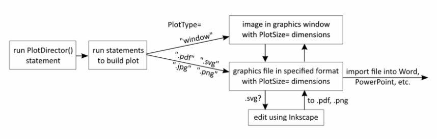
RStudio is a first-class front-end to R, but (in my opinion) its Plot pane can often be a pain. PlotDirector() quickly tells R how to format a plot with specific dimensions, either displaying it in a graphics window common to the operating system (Windows, Mac OS X, or Linux) or building a PDF, JPG, PNG, or SVG file that can be imported directly into applications such as Inkscape, PowerPoint, Word, and website development tools.
Click here to view a video showing how PlotDirector() works with Inkscape and Word.
PlotDirector() enables producing high-quality R graphics.
Arguments
PlotType="window" {=".pdf", =".svg", =".png", =".jpg"}
- ="window" opens window separate from RStudio and builds plot therein.
- =".pdf", =".svg", =".png", =".jpg" builds a disk file of the plot in the specified format. PDF files are vector graphics, so they keep their integrity when resized; they can be imported into a myriad of applications. SVG is the native format for Inkscape, a free, powerful, scalable vector graphics editor for Windows, Mac OS X and Linux. When a plot needing some tweaking, use Inkscape. For bitmap graphics, PNG is deemed better than JPG in most cases.
Quality=1.00 {0.10-1.00}
- relative pixel density for PNG and JPG.
Directory=NA {= "<path to EXISTING directory>"}
- If =NA, file is placed in current working directory. In RStudio, the current working directory can be set using Session --> Set Working Directory. Otherwise, Directory= "<path to EXISTING directory>"
- Examples:
(Mac OS) Directory="/Users/ralph/RfuncsProject/GraphicsOut"
(Linux) Directory="/home/ralph/RfuncsProject/GraphicsOut"
Filename=NA {=<a filename>}
- If =NA, set to "plot_YYMMDD.HHMMSS", where YYMMDD is the current date and HHMMSS is the current time, if it was produced on 29 February 2016 at 10:06:42, then Filename="plot_20160229.100642". The appropriate suffix is added, e.g. ".pdf".
- = "<a filename>" for PDF/JPG/PNG/SVG plot, without suffix.
- Note: The file specified must not be in use by R or any other application.
PlotSize=list(w=5, h=4)
- Width and height of plot image, in units of inches (default) or centimeters; see Units=.
Units="inches" {= "cm }
- "inches" (default) or "cm" (centimeters).
CloseOld=FALSE {=TRUE}
- =TRUE will close all existing external graphics windows.
Print=FALSE {=TRUE}
- =TRUE to print non-error messages.
Examples
<1> View a Plot
Use PlotDirector() to open an independent window and then display a scatterplot of N = 200 pairs of points, (X1, X2), having a sample correlation of 0.43. One outlier was built in. See screenshot below.
> set.seed(123)
> Z1 <- rnorm(199,0,1)
> Z2 <- 0.45*Z1 + sqrt(1-0.45^2)*rnorm(199,0,1)
> X1 <- c(50 + 7*Z1, 50 + 7*(-2.2))
> X2 <- c(130 + 20*Z2, 130 + 20*2.3)
>
> mean(X1); sd(X1)
[1] 49.9045
[1] 6.665444
> mean(X2); sd(X2)
[1] 130.9969
[1] 20.3071
> cor(X1,X2)
[1] 0.427654
> # Show plot in separate window appropriate for the operating system.
> PlotDirector(PlotSize=list(w=5,h=5,units="in."))
External graphics window opened.
Too close all such windows, use "graphics.off()"
> plot(X1,X2)
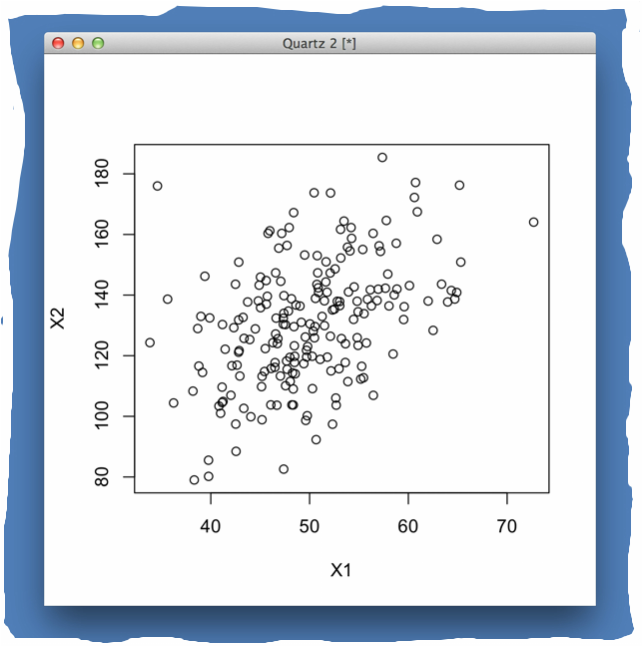
Screenshot: PlotDirector(PlotSize=list(w=5,h=5,units="in.")); plot(X1,X2)
<2> Create SVG File of Plot
Build a .svg scalable vector graphics file, which can be imported directly into Inkscape to make detailed refinements "by hand" in a GUI WYSIWYG manner. After perfecting the plot, have Inkscape save it in a more common format, such as PDF or PNG. See video.
> (originalWD <- getwd()) # Original working directory; see final statement.
[1] "/Users/ralph.../RfuncsProject"
> # This next statement gives my path. You must specify yours.
> # Or you can just set
> # GraphicsOut <- NA
> # and the PDF/SVG/JPG/PNG files will be saved in your current working
> # directory.
> GraphicsOut <- "/Users/ralph.../RfuncsProject/GraphicsOut"
> PlotDirector(PlotType=".svg", Filename="PlotDirectorExample",
+ Directory=GraphicsOut,
+ PlotSize=list(w=5,h=5,units="in."))
IMPORTANT: After creating your .svg file, run
dev.off()
to close it.
ALSO: PlotDirector() has reset your working directory to
/Users/ralph.../RfuncsProject/GraphicsOut
After plotting, to reset it as it was, enter
setwd("/Users/ralph.../RfuncsProject")
> plot(X1,X2)
> dev.off()
quartz
2
> setwd(originalWD); getwd()
# [1] "/Users/ralphobrienCWRU_MBPro07/RfuncsProject"
Video
Click here to view a video showing how PlotDirector() works with Inkscape and Word. It covers how to:
Click here to view a video showing how PlotDirector() works with Inkscape and Word. It covers how to:
- use PlotDirector to create an SVG file,
- edit it with Inkscape,
- save it as a PDF file, and
- import it into Microsoft Word.
