LogNormal()
Based on the median and relative spread, generates random values ($y), cumulative probabilities ($p.y), quantiles ($q.y), and densities (d.y) for the
logNormal() distribution. Also prints and returns various features of the distribution, including its mean, mode, standard deviation, skewness,
kurtosis, and coefficient of variation.
Nothing is "wrong" with R's built-in functions rlnorm(), plnorm(), qlnorm(), and dlnorm()—in fact, LogNormal() calls them—but they require specifying
meanlog = mean(log(Y)) for the central tendency and sdlog = sd(log(Y)) for the spread. These are abstruse for most people.
Instead:
For the central tendency, LogNormal() requires specifying
For example (#1 below),
LogNormal(Median=10, RelSpread=4)
returns values of 20 and 5 for the 0.975 and 0.025 quantiles. Thus,
LogNormal(Median=10, Quantile=20, P=0.975)
LogNormal(Median=10, Quantile=5, P=0.025)
returns results identical to LogNormal(Median=10, RelSpread=4).
Based on the median and relative spread, generates random values ($y), cumulative probabilities ($p.y), quantiles ($q.y), and densities (d.y) for the
logNormal() distribution. Also prints and returns various features of the distribution, including its mean, mode, standard deviation, skewness,
kurtosis, and coefficient of variation.
Nothing is "wrong" with R's built-in functions rlnorm(), plnorm(), qlnorm(), and dlnorm()—in fact, LogNormal() calls them—but they require specifying
meanlog = mean(log(Y)) for the central tendency and sdlog = sd(log(Y)) for the spread. These are abstruse for most people.
Instead:
For the central tendency, LogNormal() requires specifying
- the median (which is identical to the geometric mean).
- the P*100% relative spread, which for P = 0.95 (default) is the ratio of the 0.975 and 0.025 quantiles,
- the P quantile of Y, which for P = 0.95 (default) is the 0.95 quantile, i.e., the 95-th percentile.
For example (#1 below),
LogNormal(Median=10, RelSpread=4)
returns values of 20 and 5 for the 0.975 and 0.025 quantiles. Thus,
LogNormal(Median=10, Quantile=20, P=0.975)
LogNormal(Median=10, Quantile=5, P=0.025)
returns results identical to LogNormal(Median=10, RelSpread=4).
- Current (first) version released 03 February 2018.
- Download LogNormal.Rfunc180303.R
Arguments
Median
Must specify either RelSpread= or Quantile=.
RelSpread=NA
Median
- Median of Y ~ logNormal. Same as the geometric mean. Required.
Must specify either RelSpread= or Quantile=.
RelSpread=NA
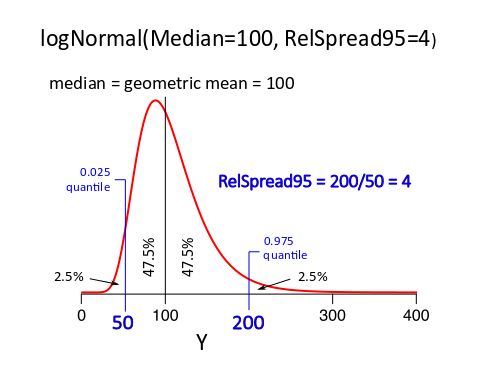
- Ratio of the 0.50 + P/2 quantile and the 0.50 - P/2 quantile. For P=0.95 (default), RelSpread ("RelSpread95") is the ratio of the 0.975 quantile and the 0.025 quantile, i.e., the ratio of the upper to the lower ends of the middle of 95% of the distribution. For P = 0.90, RelSpread is the ratio of the upper to the lower ends of the middle of 90% of the distribution.
- P quantile value of Y ~ logNormal. For P=0.95 (default), Quantile= is the 0.95 quantile, i.e. the 95-th percentile of Y ~ logNormal. For P = 0.05, Quantile= would be the 0.05 quantile.
- Defines RelSpread.
- Object of quantile levels, Q = c(value1, value2, ...), where all values are between (0, 1). Q=c(0.90, 0.95, 0.99) requests computing the 90%, 95%, and 99% quantiles (90-th, 95-th, and 99-th percentiles) of Y ~ logNormal(Median, RelSpread95).
- Object of Y values, Y = c(value1, value2, ...), where all values are positive. Q= and Y= cannot both be non-NA.
- N > 0, causes N random numbers to be generated. If so, requires Q=NA and Y=NA.
- Print=FALSE suppresses printing distribution features.
Table of Functionality
_____________________________________________________________________________________
Example Q= Y= N= Result
1 NA NA NA Prints/returns only distribution features.
2 NA NA >0 Returns N random Ys (as $y).
3 c(...) NA ignored Based on Q=, returns $y and densities ($f.y)
4 & 5 NA c(...) ignored Based on Y=, returns quantiles ($y.q) and $f.y.
_____________________________________________________________________________________
Objects Returned in List
$mean.logY .... mean of log(Y).
$SD.logY .... standard deviation of log(Y).
$mean .... mean of Y ~ LogNormal().
$median .... Median=, as specifiied.
$mode .... mode of Y ~ LogNormal().
$RelSpread95 ... ratio of 0.975 and 0.025 quantiles of Y ~ LogNormal().
$SD .... standard deviation of Y ~ LogNormal().
$CV .... coefficient of variation of Y ~ LogNormal(). $CV = $SD/$mean.
$skewness .... skewness of Y ~ LogNormal().
$kurtosis .... kurtosis of Y ~ LogNormal(). (Y ~ Normal kurtosis is 0.)
$y .... Y= (as input) or N random values, Y ~ LogNormal().
$q.y .... quantiles for Y ~ LogNormal() based on Q=.
$p.y .... Prob[Y <= y] for all values in Y= (as input).
$d.y .... densities based on Y= or Q=.
Examples
These examples are given in the "RunExamples" block of code in LogNormal().
Example 1a. Characteristics of logNormal(Median=10, RelSpread95=3).
These examples are given in the "RunExamples" block of code in LogNormal().
Example 1a. Characteristics of logNormal(Median=10, RelSpread95=3).
> Ex1 <- LogNormal(Median=10, RelSpread=4)
Median: 10.0
Mean: 10.6
Mode: 8.82
Relative spread (P = 0.95): 4.00
Standard deviation: 3.89
Coefficient of variation (SD/mean): 0.365
Skewness: 1.14
Kurtosis: 2.41 (vs. 0.00 for Normal distribution)
Quantiles
*********
0.025 0.050 0.100 0.500 0.900 0.950 0.975
5.00 5.59 6.36 10.00 15.73 17.89 20.00
Example 1b. Same distribution as Ex1a, but specified using Quantile=.
> Ex1b <- LogNormal(Median=10, Quantile=20, P=0.975)
> Ex1c <- LogNormal(Median=10, Quantile=5, P=0.025)
Both give results identical to (1a) LogNormal(Median=10, RelSpread=4)
Example 1c. Test by comparing results to a simulation.
> # Install "moments" package.
> if (!("moments" %in% .packages())) {
+ tryCatch(require("moments"),
+ warning=function(e) {
+ stop('The "moments" package is not installed.')
+ })
+ }
>
> set.seed(180128)
> y <- rlnorm(1000000, Ex1a$mean.logY, Ex1a$SD.logY)
> data.frame(TrueMedian=Ex1a$median, SimMedian=median(y),row.names="")
TrueMedian SimMedian
10 9.995748
> data.frame(TrueMean=Ex1a$mean, SimMean=mean(y),row.names="")
TrueMean SimMean
10.64532 10.6419
> data.frame(TrueRelSpread95=Ex1a$RelSpread95,
+ SimRelSpread95=qy[2]/qy[1],row.names="")
TrueRelSpread95 SimRelSpread95
4 4.000406
> data.frame(TrueSD=Ex1a$SD, SimSD=sd(y),row.names="")
TrueSD SimSD
3.88559 3.881884
> data.frame(TrueSkewness=Ex1a$skewness, SimSkewness=skewness(y),row.names="")
TrueSkewness SimSkewness
1.143642 1.142866
> data.frame(TrueKurtosis=Ex1a$kurtosis, SimKurtosis=kurtosis(y),row.names="")
TrueKurtosis SimKurtosis
2.412403 2.429231
Example 2. Generating data.
> set.seed(170322)
> Ex2 <- LogNormal(Median=100, RelSpread=4, N=7,Print=FALSE)
> y <- round(Ex2$y,2)
> # Check:
> set.seed(170322)
> ..rlnorm <- round(rlnorm(7,Ex2$mean.logY, Ex2$SD.logY),2)
> data.frame(y, ..rlnorm)
y ..rlnorm
1 92.03 92.03
2 183.91 183.91
3 74.24 74.24
4 115.80 115.80
5 83.68 83.68
6 146.07 146.07
7 92.47 92.47
Example 3. Obtaining Ys for a set of Qs.
> Q.Ex3 <- c(0.001,0.01,0.05,0.50,0.95,0.99,0.999)
> Ex3 <- LogNormal(Median=100, RelSpread=4, Q=Q.Ex3,Print=FALSE)
> q.y <- round(Ex3$q.y,1)
> # Check:
> ..q.lnrom.y <- round(qlnorm(Q.Ex3, Ex3$mean.logY, Ex3$SD.logY),1)
> data.frame(q.y, ..q.lnrom.y, row.names=Q.Ex3)
q.y ..q.lnrom.y
0.001 33.5 33.5
0.01 43.9 43.9
0.05 55.9 55.9
0.5 100.0 100.0
0.95 178.9 178.9
0.99 227.7 227.7
0.999 298.3 298.3
Example 4. Obtaining cumulative probabilities for set of Ys.
Example 4. Obtaining cumulative probabilities for set of Ys.
> Y.Ex4 <- (1:13)*25
> Ex4 <- LogNormal(Median=100, RelSpread=4, Y=Y.Ex4,Print=FALSE)
> p.y <- round(Ex4$p.y,5)
> # Check:
> ..plnorm <- round(plnorm(Y.Ex4,Ex4$mean.logY, Ex4$SD.logY),5)
> data.frame(p.y, ..plnorm, row.names=Y.Ex4)
p.y ..plnorm
25 0.00004 0.00004
50 0.02500 0.02500
75 0.20798 0.20798
100 0.50000 0.50000
125 0.73597 0.73597
150 0.87421 0.87421
175 0.94322 0.94322
200 0.97500 0.97500
225 0.98908 0.98908
250 0.99521 0.99521
275 0.99788 0.99788
300 0.99905 0.99905
325 0.99957 0.99957
Example 5. Using logNormal() to model U.S. annual family income.
The logNormal is sometimes used to model distributions of income and wealth in populations. The U.S. Census Bureau published these percentiles for household income in 2016 (unit: $1000):
10th .... 13.6
20th .... 24.0
40th .... 45.6
50th .... 59.0
60th .... 74.9
80th .... 121.0
90th .... 170.5
95th .... 225.3
--------
Source: Semega, J., Fontenot, K., and Kollar, M. (2017). Income and Poverty in the United States: 2016. Technical Report P60-259, U.S. Census Bureau, www.census.gov/content/dam/Census/library/publications/2017/demo/P60-259.pdf.
> Ex5 <- LogNormal(Median=59.0, Quantile=225.3, P=0.95,
+ Q=c(0.025,0.05,0.10,0.20,0.40,0.50,0.60,0.80,0.90,0.95,0.975))
Median: 59.0
Mean: 82.2
Mode: 30.4
Relative spread (P = 0.95): 24.4
Standard deviation: 79.8
Coefficient of variation (SD/mean): 0.970
Skewness: 3.83
Kurtosis: 34.2 (vs. 0.00 for Normal distribution)
Quantiles
*********
0.025 0.050 0.100 0.200 0.400 0.500 0.600 0.800 0.900 0.950 0.975
12.0 15.5 20.8 29.7 48.0 59.0 72.5 117.1 167.6 225.3 291.2
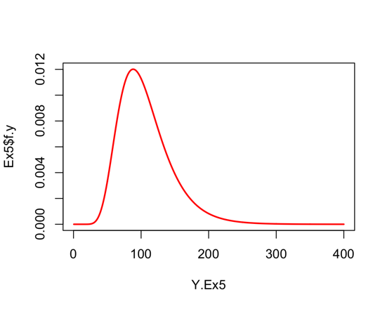
Example 6. Plotting density for Example 5.
The logNormal model for U.S. households' incomes in 2016 can be plotted with the following code. The Rfunc PlotDirector() was used to direct R to build the plot as a Scalable Vector Graphics (SVG) file called "LogNormalEx6Plot.svg" and write it to an existing directory (folder) called "RGraphics" in the current working directory.
> Ex6 <- LogNormal(Median=Ex5$median,RelSpread=Ex5$RelSpread95,
+ Q=(1:9902)/10001, Print=FALSE)
> # The next block of three statements produces and saves the plot as a .svg
> # graphics file, which can then be tweaked using Inkscape (free,
> # https://inkscape.org/en/). Of course, these paths and fileanmes are for me
> # only.
> wd <- getwd()
> dir <- paste(wd,"/RGraphics",sep="")
> PlotDirector(PlotType=".svg",Directory=dir,Filename="LogNormalEx6Plot")
> # Build plot.
> plot(Ex6$q.y,Ex6$d.y,type="l",lwd=2,col="red",bty="n",
+ xaxt="n", yaxs="i", yaxt="n", ylab="",
+ xlab="Annual Household Income (x$1000)",font.lab=2,cex.lab=1.1)
> axis(side=1, at=seq(0,400,50))
> lines(x=c(59,59), y=c(0,0.85*max(Ex6$d.y)), col="blue")
> text(59, 0.85*max(Ex6$d.y),"median: $59,000",pos=4, col="blue")
> lines(x=c(225.3,225.3), y=c(0,0.25*max(Ex6$d.y)), col="blue")
> text(225.3, 0.25*max(Ex6$d.y)," 95-th percentile: $225,300",pos=3,
+ col="blue")
Rough plot of LogNormal(Median=100, RelSpread95=5)
Note. This plot was also saved as a .svg file and customized using Inkscape, as described elsewhere on this site. The result is the graphic placed at the top of this page. See Rfunc file for code.
