MeanExp()
Maximum likelihood estimate, confidence interval, and hypothesis testing for the mean of X ~ exponential(rate=1/TrueMean), perhaps with Type II right censoring. X often represents a "survival" time, how long it takes for a specific event to occur, e.g., for a device to fail (Example 2). In Type II censoring, N independent devices may start accruing time simultaneously, but the study will stop as soon as R (≤ N) devices fail, where N and R are predetermined.
Example 2 presents an in-depth sample-size analysis with a realistic (albeit fictitious) storyline.
- Current version released 25 January 2017.
- Download CI.MeanExp.Rfunc170125.R
Arguments
Xtotal=NA
- Total of all N values of X (survival times). The first R Xs, sorted, are X.1 ≤ X.2 ≤ ... ≤ X.R. The remaining N-R Xs are all Type-II censored and have values X = X.R. Thus, Xtotal = X.1 + X.2 + ... + X.R + (N-R)*X.R. See Example 1a.
- Number of uncensored Xs, R ≤ N.
- At least R individual X values. If R is specified, then only the lowest R Xs will be used. If R = NA, then all Xs are taken to be uncensored and R is set to length(X). See Example 1b.
- Number of cases, both uncensored and Type II censored.
- Confidence level.
- ="2" for bounds of regular two-sided CI for the mean; returns c(ci["lower"], ci["upper"])
="L" for lower bound of one-sided CI for the mean; returns ci["lower"]. Upper bound is infinity.
="U" for upper bound of one-sided CI for the mean: ci["upper"]. Lower bound is 0.
- If NullMean > 0, computes the exact p-value for the test of
H0: mean = NullMean.
The sidedness of the test is set by CIbounds=, thus making the p-value congruent with the CI. See Example 3.
- To suppress printing, use Print=FALSE.
The task is sufficiently defined using one of these sets of specifications:
- Xtotal= and R=. N not relevant.
- X only. R = N = length(X)
- X= and N=. If N >= length(X), then R = length(X).
- X= and R=. If R <= length(X), then N = length(X).
- X=, R=, and N=.
Objects Returned
A list with objects
✦ CIbounds="L" returns c(ci["lower"], ci{"upper"]=Inf)
✦ CIbounds="U" returns c(ci["lower"]=0, ci{"upper"])
A list with objects
- mean ... estimated mean.
- ci ... CI.level*100% confidence limits for the mean.
✦ CIbounds="L" returns c(ci["lower"], ci{"upper"]=Inf)
✦ CIbounds="U" returns c(ci["lower"]=0, ci{"upper"])
- pvalue ... pvalue for test of H0: mean = NullMean with sidedness
congruent with type of confidence interval ("2", "L", "U")
Method
Standard theory; see Lawless, JF (1982), Statistical Models and Methods for Lifetime Data, Wiley, p. 100-103.
Standard theory; see Lawless, JF (1982), Statistical Models and Methods for Lifetime Data, Wiley, p. 100-103.
Examples
These examples are extracted from the "RunExamples" block of code in MeanExp().
Example 1: Basic use.
From Lawless (1982). p. 103:
These examples are extracted from the "RunExamples" block of code in MeanExp().
Example 1: Basic use.
From Lawless (1982). p. 103:
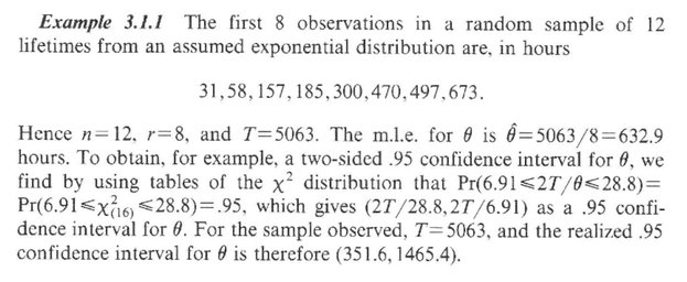
Example 1a. The total time of T = 5063 is the sum of the 8 uncensored lifetimes, plus 4*673 to include the 4 Type-II right censored lifetimes. (Because "T" is the abbreviation for "TRUE" in R, I made this argument "Xtotal".)
> Ex1a <- MeanExp(Xtotal=5063,R=8,CI.level=0.95)
Estimated mean: 633
95.0% confidence limits for the mean
------------------------------------
lower upper
351 1466
Note: The Rfuncs file delineates how mere rounding errors account for the slight discrepancies between Lawless's results and Mean.Exp's results.
This being a study of lifetime, a more meaningful CI might be one that gives only the lower bound--how short the lifetime may be.
> MeanExp(Xtotal=5063,R=8,CI.level=0.95,CIbounds="L")
Estimated mean: 633
95.0% confidence limits for the mean
------------------------------------
lower upper
385 Inf
Example 1b. This call to MeanExp uses the actual 8 uncensored values.
> lifetime <- c(31,58,157,185,300,470,497,673)
> MeanExp(X=lifetime,N=12,CI.level=0.95)
Estimated mean: 633
95.0% confidence limits for the mean
------------------------------------
lower upper
351 1466
Example 2: Statistical planning involving an exponential lifetime.
Background. The Tomedison Alternator Company (TAC) claims that its Rely90 90-amp automotive alternator has an mean lifetime of more than 5000 hours. Over the past five years, the Rely90 has been installed in over 6 million cars and small trucks produced by numerous manufacturers.
The False Claims Counter Group (FCCG) is a non-profit consumer advocacy association that discovers deceptive claims in business and industry and then sues for damages using class action lawsuits. In response to over 200
complaints from consumers about Rely90 alternators failing early in their vehicles' lifetime, the FCCG has filed suit in federal court against TAC and its allied automakers. In preparation for a settlement or eventual trial, the FCCG needs to possess strong evidence that the mean time to failure--instead of being 5000 hours as TAC has long claimed--is actually less than 4000 hours. At this stage, FCCG personnel believe the mean is likely below 3000.
FCCG has contracted with a third party to conduct a rigorous study to formally estimate the mean time to failure and to compute the associated 95% confidence interval. A judge rules that TAC must fully cooperate and provide new Rely90 units for testing at the marginal cost of production, which is 20% of retail.
Study Design. At TAC’s main warehouse, a researcher will randomly select N new Rely90 units. Each will be driven by a rubber belt attached to an electric motor that is controlled by a computer, which will vary the alternator's RPMs and also record the amperages generated. To better simulate normal use, each unit will be idled 5 times per day for 20 minutes (1.67 hours per day).
When an alternator's output falls below 50% of its nominal rating, the total time-to-failure will be recorded and that alternator will later be "autopsied” to establish the cause.
All N alternators will begin the test at the same time. When R of them have failed, the study will end with the remaining N-R alternators will be stopped before waiting for them to fail. The estimate and two-sided 95% CI for mean time-to-failure will be computed as per Lawless (1982, Section 3.1.1.). What should N and R be? That decision is critical and must be set a priori.
Rationale for planning scenario. Suppose--as FCCG believes--that the mean time-to-failure is 3000 hours, which is about 134 days running 22.33 hrs/day. As per many elementary examples in reliability testing, let's model X =
time-to-failure as an exponential random variable with a failure rate 1/4000 per hour (even though this pretends there is a constant hazard rate). Consider N = 75. If so, how many will fail within 270 days?
First things.
> TrueMean <- 3000
> N <- 75
Find the probability a given unit will fail within 270 days when run 22.33 hrs/day.
> (ProbFail.270 <- pexp(270*22.33,1/TrueMean))
[1] 0.8659711
Let #fail be the number of failures within 270 days. Find the minimum value of R such that Pr[#fail <= R | N, ProbFail.270] > 0.10.
> (R <- qbinom(p=0.10, size=N, prob=ProbFail.270))
[1] 61
Compute the probability that at least R = 61 of N = 75 units will fail within 270 days.
> round(1-pbinom(q=R-1, size=N, prob=ProbFail.270),3)
[1] 0.929
Planning questions. It is not sufficient to merely obtain a 95% confidence interval that falls completely below TAC's claim of 5000 hours. Instead, the FCCG needs to argue convincingly that the mean time-to-failure is less than 4000 hours. If the true mean is 3000 hours, what is the chance the obtained 95% CI will fall below 4000? This is the "crucial" power of this study. In addition, how precise (narrow) will the CI be?
Monte Carlo methods. These issues are herein addressed using Monte Carlo simulation. 10,000 trials provides accuracy close enough to exact for almost any purpose. (Even running 100,000 trials took only 8.5 seconds on a 2013 MacBook Pro with a 2.6 GHz processor.)
For each trial, the following block of code generates N independent time-to-failures, X,which is distributed as an exponential random variable with a mean of TrueMean = 3000 hours. It then executes MeanExp() to get the sample mean and confidence limits, and stores that trial's results. The initial study design uses N = 75 and R = 61 and computes 0.95 CIs. Note the commented statements; when executed, they change the design to N = 150, R = 124 and the CI level to 0.90.
TrueMean <- 3000;
N <- 75; R <- 61 # "N=75, R=61" study
# N <- 150; R <- 124 # "N=150, R=124" study
ci.level <- 0.95
# ci.level <- 0.90
Ntrials <- 10000
set.seed(123357)
smean <- numeric(Ntrials)
sCI <- matrix(NA,nrow=Ntrials,ncol=2,
dimnames=list(1:Ntrials,c("lower","upper")))
for (i in 1:Ntrials) {
x <- rexp(n=N, rate=1/TrueMean)
x.R <- sort(x)[1:R]
Xtotal <- sum(x.R) + (N-R)*x.R[R]
results <- MeanExp(Xtotal=Xtotal,R=R,CI.level=ci.level,Print=FALSE)
smean[i] <- results$mean
sCI[i,] <- results$ci
}
Analysis of Monte Carlo data.
- What is the probability that the estimated mean is less than 4000?
> round(sum(smean < 4000)/Ntrials,3)
[1] 0.991
- Mean confidence limits.
> round(colMeans(sCI))
lower upper
2371 3924
- Traditional power: What is the probability that the CI will be completely below TAC's claim of 5000 hours?
> round(sum(sCI[,2] < 5000)/Ntrials,3)
[1] 0.976
- Crucial power: What is the probability that the CI will be completely below 4000 hours?
> round(sum(sCI[,2] < 4000)/Ntrials,3)
[1] 0.581
Key findings, N=75, R=61, CI.level = 0.95. Under the scenario that the mean time-to-failure is 3000 hours, the design of N = 75 and R = 61 provides high traditional power (0.976). However, there was only a 0.58 crucial power for obtaining an upper confidence limit for the 95% CI that falls below 4000. The average 95% CI limits were [2371, 3924], a spread that may be too wide to be convincing at face value.
Narrowing the CI spread to produce greater power. Why must this use a 0.95 confidence level? A 0.90 level is still quite sufficient for almost all civil (non-criminal) legal cases in the United States, because they are decided based on the "preponderance of the evidence," rather than the "evidence beyond a reasonable doubt" standard used in criminal cases. 90% CIs are narrower than 95% CIs, so they also yield greater power. (This is the classic trade-off between Type-I and Type-II error rates.)
Keeping N = 75 and R = 61, but using a 90% CI produced the second set of results above. The average 0.90 confidence limits are better, [2461, 3756], as is the crucial power, 0.706. Yet this plan probably still has too much chance of producing weak results.
Doubling the sample size. What if the sample size is doubled to N = 150? The full example in the MeanExp() Rfuncs file, shows that R = 124 will be reached within 270 days with probability 0.93. For a 90% CI, the average
limits narrow to [2604, 3501], which increases the crucial power to 0.94.
A 0.90 confidence interval of [2604, 3501] would provide persuasive evidence that the lifetime mean for the Rely90 alternator is considerably below TAC's claim of a 5000-hour mean lifetime. Even [2974, 3999] would be a persuasive 90% CI. Using N = 150 and R = 124, such an interval or one even further below 5000 hours is guesstimated to happen with probability 0.94.
Summary of key Monte Carlo results:
N R Conf. Level Mean Conf. Limits Crucial Power
75 61 0.95 [2371, 3924] 0.581
75 61 0.90 [2461, 3756] 0.706
150 124 0.90 [2604, 3501] 0.938
The Rfuncs file gives the code for all these calculations.
Example 3: Does the Rely90 have a mean lifetime less than 4000 hours?
Suppose the False Claims Counter Group (FCCG) runs the N=150, R=124, CI.level=0.90 study vetted in Example 2. Also suppose the population mean lifespan of the Rely90 is not 3000 hours as per the scenario for the statistical planning, but rather is actually 3423.32 hours.
> set.seed(79838379) # Change this seed value to run other studies.
> TrueMean <- 3423.32
> N <- 150; R <- 124
> lifetime <- sort(rexp(n=N, rate=1/TrueMean))[1:R]
> MeanExp(X=lifetime,N=N,CI.level=0.90,NullMean=4000,CIbounds="2")
Estimated mean: 3387
90.0% confidence limits for the mean
------------------------------------
lower upper
2939 3952
P-value (H0: mean = 4000, two-sided): 0.076
Because this will be used as evidence in a civil lawsuit, the estimate of 3387 hours with a 90% CI of [2939, 3952] buttresses FCCG's claim that the mean lifetime of the Rely90 alternator is less than 4000 hours. Because p-values are so widely misunderstood and so casually interpreted, I would not report the p = 0.076 result, especially because it does fall below the exalted p ≤ 0.05 threshold.
