WMWodds()
Example 1. Replicate analysis of Newcombe (2006b)
Example 2. Data of Holmes and Williams (1954), used by Agresti (1980)
Example 3. Should "Super HDL" have been touted as effective?
Example 4. Statistical planning: Monte Carlo studies with WMWodds()
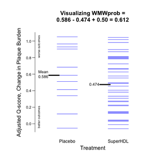
Example 5. A "congruent" plot: Using Q-scores to visualize WMWprob.
Example 6. Medians equal, yet WMWodds = 1.44, and 95% CI: [1.23, 1.68]
Example 7. Medians unequal, yet WMWodds = 1.0 & 95% CI: [0.794, 1.260]
Example 1. Replicate analysis of Newcombe (2006b)
Example 2. Data of Holmes and Williams (1954), used by Agresti (1980)
Example 3. Should "Super HDL" have been touted as effective?
Example 4. Statistical planning: Monte Carlo studies with WMWodds()
Example 5. A "congruent" plot: Using Q-scores to visualize WMWprob.
Example 6. Medians equal, yet WMWodds = 1.44, and 95% CI: [1.23, 1.68]
Example 7. Medians unequal, yet WMWodds = 1.0 & 95% CI: [0.794, 1.260]
Example 3. Should "Super HDL" have been touted as effective?
Storyline. In November 2003, Dr. Steven Nissen of the renown Cleveland Clinic Heart Center published an article in JAMA reporting his "preliminary study" that suggested improvement in atherosclerosis after only 5 weekly infusions of a manufactured experimental version of a variant in HDL cholesterol. At the time, some informally called it "Super HDL." Quoting from the article. the study "assessed the effect of intravenous recombinant ApoA-I Milano/ phospholipid complexes (ETC-216) on atheroma burden in patients with acute coronary syndromes (ACS)."
Nissen, S. E., et al. (2003). Effect of recombinant ApoA-I milano on coronary atherosclerosis in
patients with acute coronary syndromes: a randomized controlled trial. JAMA, 290(17):2292-300.
In October 2009, I wrote Dr. Nissen to obtain the data, and he initially agreed to send it, but then pulled back. Therefore, I painstakingly created a comparable dataset that gives means, medians, and SDs nearly identical to
those reported in Table 2 of the article; see below.
47 ACS patients completed the study, with
- 11 randomized to receive placebo
- 36 to receive ETC-216 ("SuperHDL")
Percent atheroma volume (PAV) is the proportion of the cardiac vessel occluded by atherosclerotic plaque. PAV.0 and PAV.5 are PAV values at Week 0 (baseline) and Week 5.
Dr. Nissen's primary outcome measure (Y) was
PAVchange = PAV.5 - PAV.0
PAVchange < 0 indicates improvement, so PAVchange = -0.04 is greater improvement than PAVchange = -0.01. A subject who goes from PAV.0 = 61.1% occlusion to PAV.5 = 55.3% occlusion has PAVchange = 55.3% - 61.1% = -5.8%, a substantial reduction (improvement) in plaque burden for only a 5-week period. Of course, this could be due to ordinary fluctuations in PAV and ever-present measurement variation. However, if SuperHDL is effective, SuperHDL subjects should tend to have lower (more negative) PAVchange scores than placebo subjects. Thus (using an obvious notation to denote the polarity of WMWodds), WMWodds[Y.placebo > Y.SuperHDL] > 1.0.
Creating the data. Code block 3.1.
> PAVchangeP <- c(-4.7,-4.0,-2.4,-1.8,-0.5,0.03,1.9,2.62,2.9,3.0,4.5)
> mean(PAVchangeP) # Table 2 in article: 0.14
[1] 0.1409091
> sd(PAVchangeP) # Table 2 in article: 3.09
[1] 3.086372
> median(PAVchangeP) # Table 2 in article: 0.03
[1] 0.03
> PAVchangeSHDL <- c(-10.0,-4.4,-4.1,-4.1,-4.1,-4.0,-4.0,-4.0,-4.0,-3.9,-3.9,
+ -3.1,-3.1,-3.0,-2.7,-2.3,-2.1,-1.02,-0.6,-0.6,-0.2,-0.1,0.8,0.9,0.9,2.1,
+ 2.2,2.2,2.2,2.2,2.2,2.4,2.5,3.0,3.8,3.9)
> mean(PAVchangeSHDL) # Table 2 in article: -1.06
[1] -1.056111
> sd(PAVchangeSHDL) # Table 2 in article: 3.17
[1] 3.174033
> median(PAVchangeSHDL) # Table 2 in article: -0.81
[1] -0.81
> treatment <- rep(c("Placebo", "SuperHDL"), c(11,36))
> PAVchange <- c(PAVchangeP, PAVchangeSHDL)
Research question. Do patients who receive Super HDL (ETC-216) tend to have lower PAVchange scores than those who receive placebo?
This question is tightly addressed by focusing on the lower confidence limit for WMWodds, i.e., a confidence interval of the form [LCL, Inf). Secondarily, the function computes the congruent one-sided p-value for testing H0: WMWodds ≤ 1 vs. H1: WMWodds > 1. This provides the essential information and increases inferential power (cuts the p-value in half), which is prudent planning for such a small ("preliminary") clinical trial.
WMWoods analysis.
> Ex3 <- WMW(Y=PAVchange, Group=treatment,
+ GroupLevel=c("Placebo", "SuperHDL"),
+ CI.type="L", H0.WMWodds=1)
*******************************************************
WMW: Wilcoxon-Mann-Whitney Analysis
Comparing Two Groups with Respect to an Ordinal Outcome
*******************************************************
WMW Parameters
**********************************************************************
WMWprob = Pr[PAVchange{Placebo} > PAVchange{SuperHDL}] +
Pr[PAVchange{Placebo} = PAVchange{SuperHDL}]/2
WMWodds = WMWprob/(1-WMWprob)
**********************************************************************
Sample Sizes
***********************
Placebo 11
SuperHDL 36
***********************
************************************************************
Stochastic Superiority # of Pairs Probability
************************** ********** ***********
{Placebo} < {SuperHDL} 151 0.381
{Placebo} = {SuperHDL} 5 0.013
{Placebo} > {SuperHDL} 240 0.606
Total: 396 1.000
WMWprob = (240 + 5/2)/396 = 0.612
WMWodds = 0.612/(1 - 0.612) = 1.58
************************************************************
*****************************************************************
Estimate 0.95 CI* H0 p**
*****************************************************************
WMWprob 0.612 [0.435, 1.000] 0.500 0.150 (one-sided)
WMWodds 1.58 [0.771, Inf] 1.00 0.150 (one-sided)
*****************************************************************
*Method based on Mee (JASA, 1990).
**P-value is congruent with both confidence intervals.
While WMWodds = 1.6 agrees suggests that SuperHDL is efficacious, the 95% lower confidence bound of 0.82 falls well short of making such an inference.
Example 5 uses $Qscores obtained from WMW() to create a Tufte-esque plot that Shows the Data for two groups through the prism of a WMW analysis. Here, too, no difference between SuperHDL and Placebo is "significantly" evident.
This analysis is markedly different from what was reported in Dr. Nissen's JAMA article. Even though its title touted this study as "a randomized controlled trial," the principal analysis ignored the placebo arm. It only assessed whether PAV improved in the SuperHDL group, a tactic disparaged routinely in better introductory texts and courses in statistical science.
WMWodds()
Example 1. Replicate analysis of Newcombe (2006b)
Example 2. Data of Holmes and Williams (1954), used by Agresti (1980)
Example 3. Should "Super HDL" have been touted as effective?
Example 4. Statistical planning: Monte Carlo studies with WMWodds()
Example 5. A "congruent" plot: Using Q-scores to visualize WMWprob.
Example 6. Medians equal, yet WMWodds = 1.44, and 95% CI: [1.23, 1.68]
Example 7. Medians unequal, yet WMWodds = 1.0 & 95% CI: [0.794, 1.260]
