WMW() ... major upgrade.
This has all been put on hold, a long story.
This WMW() documentation was under intensive development until ...
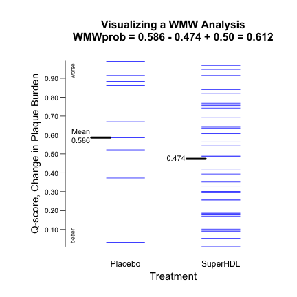 Plot of Qscores (Example 5).
The Wilcoxon-Mann-Whitney (WMW) method compares two groups with respect to an ordered categorical variable, Y. Letting Y1 and Y2 be the Y values for the two groups, the fundamental WMW parameter is
WMWprob = Prob[Y1 > Y2] + Prob[Y1 = Y2]/2
or, using odds scaling,
WMWodds = WMWprob/(1 - WMWprob).
WMW() computes the estimates and confidence intervals (two-sided or one-sided) for WMWprob and WMWodds. Optionally, setting a specific value for the null hypothesis begets a p-value congruent with the CI. The returned Qscores (transforms of Y1 and Y2) enable plotting the data in a manner consistent with WMWprob. A rich set of examples explores various applications, including performing statistical planning assessing how a planned CI might work with given research goals, study design, and total sample size.
- Current version released xx September 2018, a major upgrade..
- Download not ready
Arguments
Y
|
Required outcome variable. May have NAs.
|
Group
|
Required group variable. e.g., Group=gender. May have NAs.
|
GroupLevels = c("value1", "value2")
|
Required. Exactly two values found in the Group= variable specified above. Only cases having these two values will be used. Important: This also sets the Group order, Y1 and Y2, and thus the polarity of WMWprob and WMWodds, as defined above. Example: GroupLevels=c("m","f") defines Y1 to be outcomes for males and Y2 for females.
|
CI.type="2"
|
="2" for regular two-sided CI, [LCL, UCL], the default.
="L" for one-sided CI of the form [LCL, 1) for WMWprob; [LCL, Inf) for WMWodds. ="U" for one-sided CI of the form (0, UCL] |
Note: CI.type= also sets the type of p-value, if requested. In terms of WMWprob,
|
="2", [LCL, UCL], is congruent with H0: WMWprob = H0.WMWprob vs. H1: WMWprob ≠ H0.WMWprob.
="L", [LCL, 1.0), is congruent with H0: WMWprob ≤ H0.WMWprob vs. H1: WMWprob > H0.WMWprob. ="U", (0.0, UCL], is congruent with H0: WMWprob ≥ H0.WMWprob vs. H1: WMWprob < H0.WMWprob. |
CI.level = 0.95
|
Confidence level, between 0.00 and 1.00, but one less than 0.80 will trip a CONCERN message.
|
Method="Mee" (or "=Newcombe3")
|
="Mee", as per Mee (1990). Recommended. This is Method 6 in Newcombe (2006).
="Newcombe3", as per Newcombe's Method 3, which uses the Hanley-McNeil (1982) method coupled with Wilson's (1927) scoring CI method (instead of the Wald method). Note. Newcombe recommended his Method 5. See "Why Newcombe's Method 5 is not in WMW()" in "Beyond the Basics" below. |
H0.WMWprob=NA (e.g., H0.WMWprob=0.80)
|
Null value for testing WMWprob. Within (0,1), so not 0 or 1. The common test uses H0.WMWprob = 0.50. H0.WMWprob=and H0.WMWodds= cannot both be used. If both H0.WMWprob= and H0.WMWodds= are NA (the default), then no testing is performed.
|
H0.WMWodds=NA (e.g., H0.WMWodds=4.0)
|
Null value, positive and finite. for testing WMWodds. The common test uses H0.WMWodds = 1.0. H0.WMWodds= and H0.WMWprob= cannot both be used. If both H0.WMWprob= and H0.WMWodds= are NA, then no testing is performed.
|
Do.wilcox.test=FALSE
|
=TRUE performs wilcox.test() in R{stats}. Rarely recommended over the superior methodology built into WMW().
|
Print=TRUE
|
=FALSE suppresses all regular printing, such as when using this function for Monte Carlo simulations.
|
PrintRawPvalue=FALSE
|
By default, p-values less than 0.001 are printed as <0.001. If PrintRawPvalue=TRUE, then they are printed to 3 significant digits, e.g., .00000123.
|
Objects Returned
A list containing
- $WMWprob ...... estimate of WMWprob.
- $SE.WMWprob ...... standard error of WMWprob.
- $CI.level .... confidence level.
- $CI.WMWprob ...... c(LCL, UCL), lower amd upper confidence limits for WMWprob.
- $WMWodds ...... estimate of WMWodds.
- $CI.WMWodds ...... c(LCL, UCL), lower amd upper confidence limits for WMWodds.
- $H0.WMWprob .... null value for hypothesis test based on WMWprob.
- $H0.WMWodds .... null value for hypothesis test based on WMWodds.
- $pvalue ...... p-value for testing H0: WMWprob = H0.WMWprob or H0: WMWodds = H0.WModds. Important: Will be regular two-sided or one-sided, as set by CI.type= specification. Default: two-sided.
- $Qscore ...... Qscores in same order as original Y=. Useful for plotting. See Example 5.
- $wilcox.test.p ...... P-value from wilcox.test(), if Do.wilcox.test=TRUE.
The WMW test is (almost always) an untenable basis for comparing two medians
It is widely believed that the Wilcoxon-Mann-Whitney (WMW) test is a sound basis for testing the equality of two medians. The idea was seductive and remains so: Take a sound distribution-free test to compare the magnitudes of Y1 and Y2 and adapt it to compare their medians. Unfortunately, the strategy requires depending entirely on meeting a key theoretical assumption that is almost always untenable in practice.
Let the difference between true medians be ∆(0.50) = Q1(0.50) – Q2(0.50), where Q(0.50) denotes the 0.50 quantile (50th percentile). Hodges and Lehmann (1963) and Lehmann (1963) provided the estimates and confidence intervals for ∆(0.50) that are still widely promoted and used; e.g. see Freidlin and Gastwirth (2000) and Kloke and McKean (2015, Section 3.2.2). Today’s major statistical software systems still perform it, including wilcox.test() in R and NPAR1WAY in SAS. Unfortunately, important contradictions and its lack of consistency render this a failed method for general use.
The validity of the WMW test for comparing medians rests on the location-shift model, which pretends that the two parent distributions, F1(y) and F2(y) are identical in every way except for a difference in their medians, i.e., F1(y) = F2(y + ∆). When the model holds, it is easily shown that ∆ is also the difference between the two means and between any two like quantiles, i.e., ∆(τ) = Q1(τ) — Q2(τ); 0 < τ < 1.
It is difficult to imagine scenarios in which the location-shift model is valid. Consider:
- Let Y be a Likert-type ordinal measure with five categories (1, 2, 3, 4 5), as per Examples 1, 2 4, and 6. If the location-shift holds with ∆ = 1.0, then the probability structure must be:
Y: 1 2 3 4 5
Group 1 0.00 a b c d
Group 2 a b c d 0.00
where a = Pr{Y = 2 | Group 1] = Pr{Y = 1 | Group 2], etc. Such a scenario is virtually untenable.
- Suppose Y is body mass index, BMI. Let Group 1 have population quartiles of Q1(0.05) = 19.3 and Q1(0.95) = 37.2, If the population for Group 2 has much less obesity, say, Q2(0.95) = 29.7, then the location-shift model has ∆ = 7.5 BMI units. But this implies that Q2(0.05) = 19.3 – 7.5 = 11.8, which corresponds to someone 6-feet tall weighing only 87 pounds (183 cm, 39.5 kg). It is virtually untenable that 5% of some population could be so emaciated.
- Many Y measures are non-negative with Y = 0 being common, such as number of concussions suffered in a life-time. If Group 2 might have subjects who are concussion-free (Y = 0) and the location-shift is ∆ > 0, then every subject in Group 1 must have at least ∆ concussions and thus zero chance of being life-time concussion-free. This is completely untenable.
Examples 6 and 7 show concretely that the WMWprob and WMWodds parameters have no functional relationship to the difference in medians. In fact, assuming that the location-shift model holds can lead to bizarre estimates and confidence intervals for the difference in medians. Stated directly, the WMW test does not compare two medians (or any other quantile) any more than it compares two means.
So, what parameter does correspond to the Hodges-Lehmann estimator? Answer: ∆ = median(Y1 - Y2), which is another natural quantification of the difference between Y1 and Y2, and it does not rest on the location-shift model. As Lehmann summarized in his seminal 1975 book on nonparametrics, this estimator is median unbiased when n1*n2 is odd, and approximately so when n1*n2 is even. But whereas mean(Y1 – Y2) = mean(Y1) – mean(Y2), median(Y1 - Y2) ≠ median(Y1) - median(Y2) unless the troublesome location-shift model holds,
CI.WMWparms()
Example 1. Replicate analysis of Newcombe (2006b)
Example 2. Data of Holmes and Williams (1954), used by Agresti (1980)
Example 3. Should "Super HDL" have been touted as effective?
Example 4. Statistical planning: Monte Carlo studies with CI.WMWparms()
Example 5. A "congruent" plot: Using Q-scores to visualize WMWprob.
Example 6. Medians equal, yet WMWodds = 1.44, and 95% CI: [1.23, 1.68]
Example 7. Medians unequal, yet WMWodds = 1.0 & 95% CI: [0.794, 1.260]
